如何用Python找到股票的支撑位和压力位？——局部极值

大家好，我是花姐。经常有小伙伴问我：“股票的支撑位、压力位怎么找？有没有办法用 Python 程序自动算出来？”

上一篇我们讲了通过枢轴点来确定压力和支撑位置，今天我们来说说局部极值法确定压力和支撑位置。

开始前的准备

我这里用的行情数据源是 xtquant + miniQMT。 后续示例里会用到一些常见的 Python 库：pandas, numpy, matplotlib，进阶部分还会涉及 scipy, sklearn。在实际运行代码之前，记得先把环境配置好：

pip install pandas numpy matplotlib scipy scikit-learn xtquant

这样就能避免因为依赖缺失导致的报错啦。

以下是一个基于xtquant + miniQMT获取股票行情的方法，后面的行情Dataframe数据都会通过这个方法来获取：

def get_hq(code,start_date='19900101',period='1d',dividend_type='front_ratio',count=-1):
    '''
    基于xtquant下载某个股票的历史行情
    盘中运行最后一个K里存了最新的行情
    period 1d 1w 1mon
    dividend_type - 除权方式，用于K线数据复权计算，对tick等其他周期数据无效
    none 不复权
    front 前复权
    back 后复权
    front_ratio 等比前复权
    back_ratio 等比后复权
    '''
    xtdata.enable_hello = False
    xtdata.download_history_data(stock_code=code, period='1d',incrementally=True)
    history_data = xtdata.get_market_data_ex(['open','high','low','close','volume','amount','preClose','suspendFlag'],[code],period=period,start_time=start_date,count=count,dividend_type=dividend_type)
    print(history_data)
    df = history_data[code]

    df.index = pd.to_datetime(df.index.astype(str), format='%Y%m%d')
    df['date'] = df.index
    return df

1. 由来与直观理解

直观上，局部极值就是价格曲线上的“山顶”（Swing High）和“山谷”（Swing Low）。这些点往往被交易者记住，并在后续成为阻力/支撑，比如价格反复在某个高度回落或反弹。

在技术分析里，很多工具（ZigZag、Fractals）本质上都是在寻找这些极值或近似极值，用来刻画市场结构（高点更高 / 低点更高 → 上升结构，反之则为下降结构）。

2. 数学定义与原理

1. 局部最大值（order = k） 给定序列 $x_t$，索引 $i$ 是局部最大值（order=k）当且仅当：

   $$x_i>x_{i-j}\text{and}{x}_i>x_{i+j},\mathrm{\forall }j=1,\dots ,k$$

   同理，局部最小值是小于左右 k 个点的点。

2. 极值确认（实际交易中常用） 为了避免把“噪声尖刺”当做极值，通常要求在极值之后还要看到 confirm 根反方向的柱子（例如峰后连续 confirm 个低点），才把它标记为已确认的极值（避免未来回溯/偷看数据的风险）。

3. 峰的显著性（prominence） prominence（高峰显著性）衡量一个峰相对于周围基线有多“突出”。通俗说就是峰顶到比它高的最近两侧“最低包围线”的高度。数值越大，代表更显著、更值得关注（也越不易被噪声触发）。

3. 常用算法

在 Python 里，其实不用我们自己写很多复杂的逻辑，scipy 这个科学计算库已经帮我们准备好了“找高点/低点”的工具。里面常用的有两个方法：

1. argrelextrema

   • 这个名字有点拗口，但原理很直白：就是和左右的邻居比大小。
   • 比如：如果某点比左右各 3 根K线都高，那它就是一个局部高点；比左右都低，就是局部低点。
   • 参数 order 就是控制“左右要比多少根”。

2. find_peaks

   • 顾名思义，就是“找山顶”的工具。

   • 它可以找到价格曲线里的局部高点，如果把价格取负数，就能反过来找低点。

   • 还能加条件筛选，比如：

     • 两个高点之间至少要隔多少根K线（distance）；
     • 这个高点要多明显才算（prominence）；
     • 要求高点的高度（height）；
     • 要求高点的宽度（width）。

花姐实战经验：

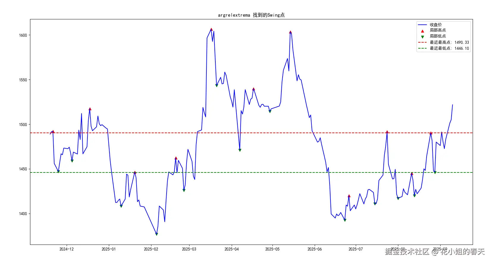
• argrelextrema 适合入门，逻辑简单直观。
• find_peaks 更强大，可以根据显著性、间隔等条件自动过滤掉很多没意义的小波动。
• 我自己常用 find_peaks + 平滑处理 + 基于 ATR 的显著性阈值，这样提取出来的高低点更稳健，不容易被噪声干扰。

4. 实战Python代码

4.1 使用argrelextrema寻找压力支撑

下面的示例代码使用了 Python 的 scipy.signal.argrelextrema 来寻找局部极值，并绘制成可视化图表。

from xtquant import xtdata
import pandas as pd
import numpy as np
import matplotlib.pyplot as plt
from scipy.signal import argrelextrema

def find_swings_argrelextrema(price_series, order=5):
    arr = price_series.values
    # 找高点（局部最大值）
    peaks_idx = argrelextrema(arr, np.greater, order=order)[0]
    # 找低点（局部最小值）
    valleys_idx = argrelextrema(arr, np.less, order=order)[0]
    return peaks_idx, valleys_idx

def plot_swings(price_series, peaks_idx, valleys_idx, title="Swing Points"):
    # 设置中文字体（SimHei = 黑体，常用）
    plt.rcParams['font.sans-serif'] = ['SimHei']  
    plt.rcParams['axes.unicode_minus'] = False  # 解决负号显示问题
    plt.figure(figsize=(12,6))
    plt.plot(price_series.index, price_series.values, label="收盘价", color="blue")
    
    
    # 标记Swing High/Low
    plt.scatter(price_series.index[peaks_idx], price_series.values[peaks_idx],
                marker="^", color="red", label="局部高点")
    plt.scatter(price_series.index[valleys_idx], price_series.values[valleys_idx],
                marker="v", color="green", label="局部低点")
    
    # 最近最高点和最低点
   
    recent_high = price_series.values[peaks_idx[-1]]
    recent_low = price_series.values[valleys_idx[-1]]
    
    plt.axhline(recent_high, color="red", linestyle="--", label=f"最近最高点: {recent_high:.2f}")
    plt.axhline(recent_low, color="green", linestyle="--", label=f"最近最低点: {recent_low:.2f}")
    
    plt.title(title)
    plt.legend()
    plt.show()

if __name__ == "__main__":
    code = '600519.SH'  # 贵州茅台
    df = get_hq(code, start_date='20200101', period='1d', count=200)
    peaks_idx1, valleys_idx1 = find_swings_argrelextrema(df["close"], order=5)
    plot_swings(df["close"], peaks_idx1, valleys_idx1, title="argrelextrema 找到的Swing点")

代码解析

1. 寻找局部高低点

peaks_idx = argrelextrema(arr, np.greater, order=order)[0]
valleys_idx = argrelextrema(arr, np.less, order=order)[0]

• arr 是价格序列（这里用 close 收盘价）。
• order 表示左右要比多少根K线才能判断为极值，比如 order=5 意味着这个点比前后各 5 根 K 线都高或都低才算极值。
• peaks_idx 存放局部高点索引，valleys_idx 存放局部低点索引。

2. 可视化

plot_swings 函数会：

• 绘制价格曲线
• 用红色三角标记局部高点，绿色倒三角标记局部低点
• 在图上画出最近的最高点和最低点水平虚线，标注价格，方便快速识别当前关键支撑/阻力。

3. 实战演示

df = get_hq(code, start_date='20200101', period='1d', count=200)
peaks_idx1, valleys_idx1 = find_swings_argrelextrema(df["close"], order=5)
plot_swings(df["close"], peaks_idx1, valleys_idx1, title="argrelextrema 找到的Swing点")

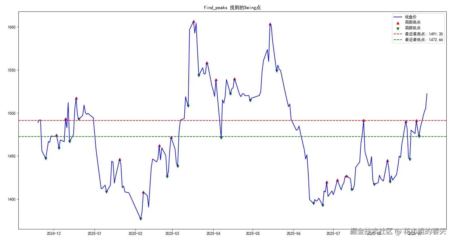
• 这里以贵州茅台 (600519.SH) 的日线数据为例，获取最近 200 根K线。
• 调用 find_swings_argrelextrema 自动识别局部极值，再通过 plot_swings 可视化。
• 图中红色水平虚线表示最近最高点，绿色水平虚线表示最近最低点，帮助直观判断当前价格位置。

4. 使用建议

• order 参数：数值越大，算法越保守，只保留显著的高低点，避免噪声影响。
• 图表仅作为参考，实际策略中通常会结合趋势、成交量或其他指标进行进一步确认。
• 对于短周期数据，建议先平滑价格序列，再找极值，以避免被小波动干扰。

4.2 使用find_peaks寻找压力支撑

下面的示例代码使用了 Python 的 scipy.signal.find_peaks 来寻找局部极值，并绘制成可视化图表。

from xtquant import xtdata
import pandas as pd
import numpy as np
import matplotlib.pyplot as plt
from scipy.signal import argrelextrema, find_peaks

def get_hq(code,start_date='19900101',period='1d',dividend_type='front_ratio',count=-1):
    '''
    基于xtquant下载某个股票的历史行情
    盘中运行最后一个K里存了最新的行情
    period 1d 1w 1mon
    dividend_type - 除权方式，用于K线数据复权计算，对tick等其他周期数据无效
    none 不复权
    front 前复权
    back 后复权
    front_ratio 等比前复权
    back_ratio 等比后复权
    '''
    xtdata.enable_hello = False
    xtdata.download_history_data(stock_code=code, period='1d',incrementally=True)
    history_data = xtdata.get_market_data_ex(['open','high','low','close','volume','amount','preClose','suspendFlag'],[code],period=period,start_time=start_date,count=count,dividend_type=dividend_type)
    print(history_data)
    df = history_data[code]

    df.index = pd.to_datetime(df.index.astype(str), format='%Y%m%d')
    df['date'] = df.index
    return df

def find_swings_findpeaks(price_series, distance=5, prominence=0.5):
    arr = price_series.values
    # 高点
    peaks_idx, _ = find_peaks(arr, distance=distance, prominence=prominence)
    # 低点（对价格取负）
    valleys_idx, _ = find_peaks(-arr, distance=distance, prominence=prominence)
    return peaks_idx, valleys_idx

def plot_swings(price_series, peaks_idx, valleys_idx, title="Swing Points"):
    # 设置中文字体（SimHei = 黑体，常用）
    plt.rcParams['font.sans-serif'] = ['SimHei']  
    plt.rcParams['axes.unicode_minus'] = False  # 解决负号显示问题
    plt.figure(figsize=(12,6))
    plt.plot(price_series.index, price_series.values, label="收盘价", color="blue")
    
    
    # 标记Swing High/Low
    plt.scatter(price_series.index[peaks_idx], price_series.values[peaks_idx],
                marker="^", color="red", label="局部高点")
    plt.scatter(price_series.index[valleys_idx], price_series.values[valleys_idx],
                marker="v", color="green", label="局部低点")
    
    # 最近最高点和最低点
   
    recent_high = price_series.values[peaks_idx[-1]]
    recent_low = price_series.values[valleys_idx[-1]]
    
    plt.axhline(recent_high, color="red", linestyle="--", label=f"最近最高点: {recent_high:.2f}")
    plt.axhline(recent_low, color="green", linestyle="--", label=f"最近最低点: {recent_low:.2f}")
    
    plt.title(title)
    plt.legend()
    plt.show()

if __name__ == "__main__":
    code = '600519.SH'  # 贵州茅台
    df = get_hq(code, start_date='20200101', period='1d', count=200)
    
    # ==== 演示 find_peaks ====
    peaks_idx2, valleys_idx2 = find_swings_findpeaks(df["close"], distance=5, prominence=5.0)
    plot_swings(df["close"], peaks_idx2, valleys_idx2, title="find_peaks 找到的Swing点")

代码解析

1. 寻找局部极值（Swing High / Low）

peaks_idx2, valleys_idx2 = find_swings_findpeaks(df["close"], distance=5, prominence=5.0)

• distance=5：控制相邻高点/低点最少间隔 5 根K线，避免捕捉太密集的小波动。
• prominence=5.0：高点或低点必须足够突出才被认为是有效极值，过滤噪声。
• 返回索引 peaks_idx2（高点）和 valleys_idx2（低点），便于后续绘图或策略使用。

2. 可视化

plot_swings(df["close"], peaks_idx2, valleys_idx2, title="find_peaks 找到的Swing点")

• 绘制收盘价曲线
• 红色三角标记局部高点（Swing High）
• 绿色倒三角标记局部低点（Swing Low）
• 图中红色虚线标出最近最高点，绿色虚线标出最近最低点，直观展示当前支撑/阻力水平。

3. 使用建议

• distance 和 prominence 参数需要根据周期和品种调节，避免噪声或错过重要波峰波谷。
• 对于短周期或高波动品种，建议先做价格平滑，再寻找极值。
• 仅靠极值做交易可能不够稳健，建议结合趋势、成交量或其他指标进一步确认。

今天关于寻找股票支撑与压力位的局部极值法就写到这里了，更高级的用法有兴趣的朋友可以结合AI来自由探索，花姐这里只做简单科普抛砖引玉。

下一篇我们介绍通过均线簇寻找股票支撑与压力位。