如何用Python找到股票的支撑位和压力位？——均线簇

匿名上传

发布时间:2025-10-07 10:30:01

大家好，我是花姐。经常有小伙伴问我：“股票的支撑位、压力位怎么找？有没有办法用 Python 程序自动算出来？”

之前我们讲了通过枢轴点、局部极值2种方法来确定压力和支撑位置，今天我们来说说均线簇法确定压力和支撑位置。

开始前的准备

我这里用的行情数据源是 xtquant + miniQMT。后续示例里会用到一些常见的 Python 库：pandas, numpy, matplotlib，进阶部分还会涉及 scipy, sklearn。在实际运行代码之前，记得先把环境配置好：

pip install pandas numpy matplotlib scipy scikit-learn xtquant

这样就能避免因为依赖缺失导致的报错啦。

以下是一个基于xtquant + miniQMT获取股票行情的方法，后面的行情Dataframe数据都会通过这个方法来获取：

def get_hq(code,start_date='19900101',period='1d',dividend_type='front_ratio',count=-1):
    '''
    基于xtquant下载某个股票的历史行情
    盘中运行最后一个K里存了最新的行情
    period 1d 1w 1mon
    dividend_type - 除权方式，用于K线数据复权计算，对tick等其他周期数据无效
    none 不复权
    front 前复权
    back 后复权
    front_ratio 等比前复权
    back_ratio 等比后复权
    '''
    xtdata.enable_hello = False
    xtdata.download_history_data(stock_code=code, period='1d',incrementally=True)
    history_data = xtdata.get_market_data_ex(['open','high','low','close','volume','amount','preClose','suspendFlag'],[code],period=period,start_time=start_date,count=count,dividend_type=dividend_type)
    print(history_data)
    df = history_data[code]

    df.index = pd.to_datetime(df.index.astype(str), format='%Y%m%d')
    df['date'] = df.index
    return df

1. 由来与直观理解

在股市里，价格上涨或者下跌往往会遇到一些“阻力”或“支撑”，这个概念大家可能听得多，但怎么量化呢？

于是就有了均线簇的概念：

我们把多条均线同时画在一张K线图上
当这些均线在某个价格区间聚集时，就形成了“均线簇”
均线簇的密集区往往对应压力位（价格上不去）或支撑位（价格不跌破）

直观理解：

想象几条橡皮筋同时捆在股票价格上方或下方，价格想突破或跌破时就像要拉开橡皮筋，会有阻力
这就是均线簇在做的事情：用过去价格的平均值，画出价格心理关口

2. 数学定义与原理

简单移动平均线（SMA）

S M A_{n} (t) = \frac{1}{n} \sum_{i = 0}^{n - 1} P_{t - i} SMA_n(t) = frac{1}{n} sum_{i=0}^{n-1} P_{t-i}

$n n$ 是窗口大小（天数）
$P_{t} P_t$ 是第 $t t$ 天的收盘价

均线簇的形成条件

当多条不同周期均线之间的价格差异非常小，比如5日、10日、20日、30日均线同时靠近同一个价格区间
数学上可以用均线标准差或者均线最大最小差值来量化：

MA_spread = \max (M A_{1}, M A_{2}, . . ., M A_{n}) - \min (M A_{1}, M A_{2}, . . ., M A_{n}) text{MA_spread} = max(MA_1, MA_2, ..., MA_n) - min(MA_1, MA_2, ..., MA_n)

当 MA_spread 很小，说明均线聚集形成簇

原理：

均线簇反映了市场短中期均衡状态
多空力量在这个价格附近相对均衡
突破均线簇往往伴随成交量放大，是典型的趋势启动信号

3. 常用算法

简单聚合均线

选择5条或以上不同周期均线
计算均线最大最小差值
小于阈值时判定为均线簇

均线簇密度算法（进阶）

用均线标准差衡量密集度：

MA_std = std (M A_{1}, M A_{2}, . . ., M A_{n}) text{MA_std} = text{std}(MA_1, MA_2, ..., MA_n)

标准差越小，均线聚集越密集
可以设置动态阈值，如过去20日均值的20%

支撑/压力判定

均线簇在股价上方 → 压力位
均线簇在股价下方 → 支撑位

4. 实战Python代码

均线簇 ≈ 市场在蓄力，方向不确定，但一旦突破，往往容易走出一波行情

4.1 使用简单聚合均线

计算思路

1 算均线 → 5日、10日、20日、30日、60日
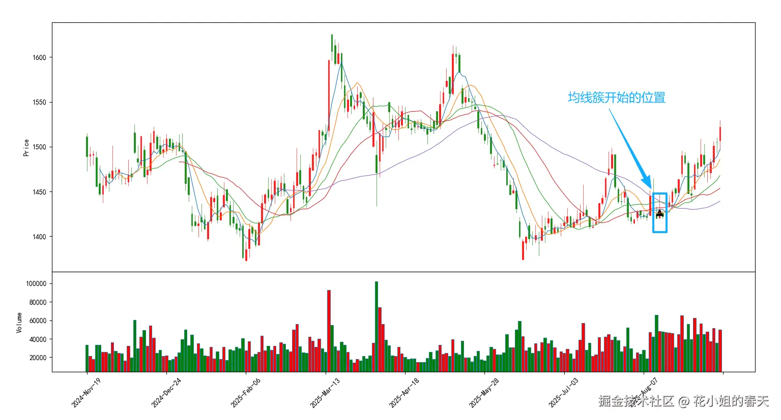
2.判断是否簇 → 如果这些均线的最高值和最低值之间的差距小于价格的1%，就算是“簇”。
3.找第一个点 → 我们只想标记簇刚出现的时候（而不是整个簇区域）。

示例代码

from xtquant import xtdata
import pandas as pd
import numpy as np
import matplotlib.pyplot as plt
import mplfinance as mpf

def detect_ma_clusters(df, ma_periods=[5, 10, 20, 30, 60], price_col='close', threshold_pct=0.01):
    """
    根据均线计算均线簇，并只返回连续簇的第一个点
    """
    df = df.copy()
    print(df)
    # 1. 计算均线
    for period in ma_periods:
        df[f'MA_{period}'] = df[price_col].rolling(window=period).mean()

    df = df.dropna(subset=[f'MA_{p}' for p in ma_periods])
    print(df)
    ma_cols = [f'MA_{p}' for p in ma_periods]

    # 2. 计算均线最大最小值及差值
    df['MA_max'] = df[ma_cols].max(axis=1)
    df['MA_min'] = df[ma_cols].min(axis=1)
    df['MA_spread'] = df['MA_max'] - df['MA_min']

    # 3. 判断均线簇（相对价格）
    df['Cluster'] = df['MA_spread'] / df[price_col] < threshold_pct

    # 4. 只取连续簇的第一个值
    # shift(1) 表示前一天的 Cluster 状态
    df['Cluster_start'] = (df['Cluster'] & ~df['Cluster'].shift(1).fillna(False))

    # 取出第一个点
    cluster = df.loc[df['Cluster_start'], price_col]

    return cluster

def draw_ma_clusters(df, cluster, ma_periods=[5, 10, 20, 30, 60]):
    # mplfinance 要求 DataFrame 索引为日期，并包含 Open, High, Low, Close
    mpf_data = df[['open','high','low','close','volume']].copy()
    mpf_data.index = pd.DatetimeIndex(mpf_data.index)
    
    apds = []
    # 准备支撑位/压力位标记
    cluster_y = np.full(len(mpf_data), np.nan)
    # 填充支撑位/压力位对应价格
    if len(cluster) > 0:
        for date, price in cluster.items():
            if date in mpf_data.index:
                idx = mpf_data.index.get_loc(date)
                cluster_y[idx] = price
        apds.append(mpf.make_addplot(cluster_y, type='scatter', markersize=80, marker='^', color='black'))
        
    mc = mpf.make_marketcolors(up='r', down='g', inherit=True)
    s  = mpf.make_mpf_style(marketcolors=mc,rc={'font.family': 'SimHei'})

    mpf.plot(
        mpf_data,
        type='candle',
        style=s,
        title="K线及均线簇",
        mav=ma_periods,
        addplot=apds,
        volume=True,
        figsize=(14,7)
    )
    

if __name__ == "__main__":
    code = '600519.SH'  # 贵州茅台
    df = get_hq(code, start_date='20200101', period='1d', count=200)
    cluster = detect_ma_clusters(df, ma_periods=[5, 10, 20, 30, 60])
    draw_ma_clusters(df, cluster, ma_periods=[5, 10, 20, 30, 60])

4.2 使用均线簇密度算法（进阶）

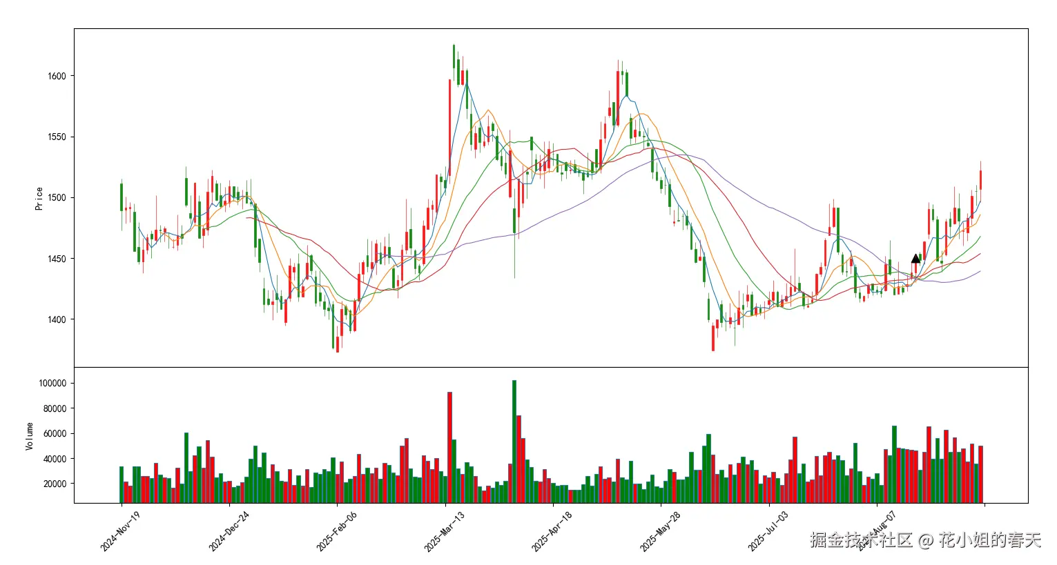
计算思路

计算不同周期的均线；
计算这些均线的标准差 MA_std；
用动态阈值：MA_std < rolling_mean(MA_std, 20) * factor 来判定是否属于“均线簇”；
依然只取连续簇的第一个点。

示例代码

from xtquant import xtdata
import pandas as pd
import numpy as np
import matplotlib.pyplot as plt
import mplfinance as mpf

def draw_ma_clusters(df, cluster, ma_periods=[5, 10, 20, 30, 60]):
    # mplfinance 要求 DataFrame 索引为日期，并包含 Open, High, Low, Close
    mpf_data = df[['open','high','low','close','volume']].copy()
    mpf_data.index = pd.DatetimeIndex(mpf_data.index)
    
    apds = []
    # 准备支撑位/压力位标记
    cluster_y = np.full(len(mpf_data), np.nan)
    # 填充支撑位/压力位对应价格
    # 支撑位绘制
    if len(cluster) > 0:
        for date, price in cluster.items():
            if date in mpf_data.index:
                idx = mpf_data.index.get_loc(date)
                cluster_y[idx] = price
        apds.append(mpf.make_addplot(cluster_y, type='scatter', markersize=80, marker='^', color='black'))
        
    mc = mpf.make_marketcolors(up='r', down='g', inherit=True)
    s  = mpf.make_mpf_style(marketcolors=mc,rc={'font.family': 'SimHei'})

    mpf.plot(
        mpf_data,
        type='candle',
        style=s,
        title="K线及均线簇",
        mav=ma_periods,
        addplot=apds,
        volume=True,
        figsize=(14,7)
    )
    
    
def detect_ma_clusters_std(df, ma_periods=[5, 10, 20, 30, 60], price_col='close', 
                       lookback=20, factor=0.2):
    """
    基于均线标准差来检测均线簇，并只返回连续簇的第一个点
    
    参数：
        df : DataFrame，行情数据
        ma_periods : list，均线周期
        price_col : str，收盘价字段
        lookback : int，动态阈值的回看窗口
        factor : float，动态阈值因子（比如0.2表示20%）
    """
    df = df.copy()

    # 1. 计算均线
    for period in ma_periods:
        df[f'MA_{period}'] = df[price_col].rolling(window=period).mean()

    df = df.dropna(subset=[f'MA_{p}' for p in ma_periods])
    ma_cols = [f'MA_{p}' for p in ma_periods]

    # 2. 计算均线标准差
    df['MA_std'] = df[ma_cols].std(axis=1)

    # 3. 计算动态阈值：过去 lookback 日 MA_std 均值 * factor
    df['Threshold'] = df['MA_std'].rolling(window=lookback).mean() * factor

    # 4. 判断均线簇
    df['Cluster'] = df['MA_std'] < df['Threshold']

    # 5. 只取连续簇的第一个点
    df['Cluster_start'] = (df['Cluster'] & ~df['Cluster'].shift(1).fillna(False))

    # 取出第一个点（收盘价作为簇的价格）
    cluster = df.loc[df['Cluster_start'], price_col]

    return cluster

if __name__ == "__main__":
    code = '600519.SH'  # 贵州茅台
    df = get_hq(code, start_date='20200101', period='1d', count=200)

    cluster = detect_ma_clusters_std(df, ma_periods=[5, 10, 20, 30, 60])
    draw_ma_clusters(df, cluster, ma_periods=[5, 10, 20, 30, 60])